Week 29 - Conditional Formatting

CLASS OBJECTIVE

Apply conditional formatting in a spreadsheet table to automatically highlight the relevant contents in a cell or a range.

INTRODUCTION

In this course we have already talked about cell formats, such as fill colors, borders, font formats, etc. Conditional formatting will AUTOMATICALLY alter the appearance of certain cells, but we must established a condition for this format to be applied.

For example, on a report card it is very common to see grades below 6 appear highlighted in red.

In this example of conditional formatting, when changing the grades below 6 to passing grades, the format should be updated automatically.

In today's activity you will have to use a table like the one above to apply these formats that will be applied when certain conditions are met.

CONDITIONAL FORMATTING

The procedure for applying conditional formatting in Google Sheets is pretty simple. As always, the main thing is to correctly select the cells in which you will apply this Conditional Formatting.

Once the selection of the cells has been made, in the FORMAT tab you have to select the CONDITIONAL FORMATTING option. This will open a new panel on the far right of the screen, like the one shown below.

 

If you correctly selected the cells before opening this panel, it will no longer be necessary to indicate where the format will be applied.

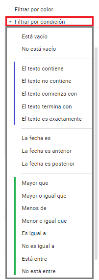
• FORMAT RULES. It is the condition that is established so that the formats are applied, for example, a number is greater or less than another, or that it contains a certain text, or that some date is met.
•  FORMATTING STYLE. They are the formats that will be applied in case the condition has been met. You will notice that they are only font or fill formats.

With the "Add another rule" button you can establish more conditional formats, but the order in which they are applied could override the previous ones.

Practice of the topic (done together with the teacher)

You should take your class notes before completing this week's activity. To do it completely, you'll need to remember several topics such as sorting, filtering, formulas, and functions (prior knowledge.

Now that we are about to close the school year, a spreadsheet report will be very useful to help you calculate your final grades and averages.

• To get started, open a new spreadsheet and you will create the following table. Apply static formats, that is, those that don't change automatically.

 

• Fill in the table with your grades from Periods 1 and 2. Make up grades for the third period.
• Calculate subject averages, period averages, maximum and minimum grade per period, using the AVERAGE, MAX and MIN functions.
• Set the "number format" so that grades are displayed with only one decimal place.
• Apply bold format to the results of the AVERAGE function.

Use this example table to compare with your results.

Now you will apply the conditional formats.

• Select the grades of all your subjects, use the following reference (C3: F13).
• Apply conditional formatting to these cells so that grades less than 6.0 have a red background and white letters.
• Now select only the results of the averages by period (C15: F15) and the averages by subject (F3: F13). Remember to use the CONTROL key to select both ranges.
• Apply conditional formatting so that grades less than 8.0 have a yellow background.

Since the grades of Period 3 are not real yet, I invite you to change them so that you can see how the format of the cells is automatically changed when the established condition is met. Make up some "under 6" grades and you will see the changes.

Week 28 - Advanced filters in the spreadsheet.

 CLASS OBJECTIVE

Apply Sorting and Filters with multiple criteria, to achieve greater precision in the organization and location of the information.

HOW TO ESTABLISH MORE THAN ONE SORTING CRITERIA

When sorting a table it is possible to use more than one criteria to arrange the records. This is very common when the data in a table is constantly repeating.

A very common example is the ordering of a school list, in which surnames are the main criteria but some of these are obviously repeated, such as García or Hernández. In these cases, a second sort criteria is used to rearrange the records that met the first criteria.

We can see another example in the following image, in which the first ordering criteria is the group, but to improve it, age was used as the second criteria and height as the third.

To add sorting criteria you will use the button marked in red.

HOW TO ESTABLISH MORE THAN ONE FILTER CRITERIA

Doing this means that we can filter a filtered table, we simply will not remove the first one.

In these cases, each time we filter the table we will have fewer records on the screen, so the filter can be used to locate information.

To show the entire table again you should deactivate ALL the filters.

FILTER BY CONDITION

There will be times when the list of items of a filter will not be enough. For this we’ll use the “Filter by Condition” option, which offers you the possibility to program the filter.

For example, we can filter by asking for the content of cells, for a word contained in them. We can also filter by asking for numerical ranges, such as "greater or less than".

Week 26/27 - Sorting and filtering a table.

 OBJECTIVE OF THE CLASS

Learn to organize information contained in a table, through the Sort and Filter tools of Google Sheets.

EXAM REVIEW Clarification of doubts, comments and important details after taking the exam and having obtained a grade. How did it go? What did you fail at? What was the most difficult? What do you think should be revised or strengthened? COVER PAGE PERIOD 3 After the review period, a short time will be determined for the creation of the cover of Period 3, which will continue with the theme of the spreadsheet with filters, sorting, logical and graphic functions, remember that the cover must use the same data than the previous period.

TABLE

We’ll call Table to a limited collection of information, stored and organized within a spreadsheet.

The line records are organized by the table headers, which we will call Fields.

For example:

In a "directory" we record the data of many persons but we write them by the headers, that is, in their corresponding field.

Name	Last Name	Age	Phone number	Municipality
Alberto	Gómez	14	3334445555	Zapopan
María	Herrera	13	3339998888	Guadalajara
Pedro	Acosta	15	3338887777	Zapopan
Ana	Valencia	14	3335556666	Tlajomulco

SORT

This is a spreadsheet tool specifically used on a data table. With it, we can place the data records according to a certain criteria, for example, ordered by surname, or by age. The order may be ascending or descending, that is, from A-Z or Z-A, from the smallest to the largest number or vice versa.

Obviously the order of the rows will be altered, but the data will not be mixed with other records.

This tool is used to organize and analyze the information contained in a table.

Look at the table above and tell: which record would be the first if the table is sorted by age in ascending order? or What would be the first if they are ordered by last name but in descending order?

To apply Sorts in Google Sheets I suggest the following procedure

1. Select the entire table, from the names of the fields to the last data.

2. Display the DATA tab and select the SORT RANGE option.

3. It will ask you if the table has headers, because it shouldn't involve them in the ordering.

4. Finally, you will choose the main Sorting criteria.

5. Optionally, you can use secondary Sortering criteria, which will be applied after the main one.

Let's do a couple of examples with the table proposed by your teacher, if the examples are done completely and correctly we will do an example of the filters tool.

FILTERS

This is another tool to analyze and locate information within a table but, unlike sorting, the filters will only show some records from the table, those that match the filter criteria.

For example, in the table above you can use filters to show only 14-year-olds. Who are they?

Another example, use a filter to show the people who live in Zapopan. Who are they?

To apply Filters in Google Sheets I suggest the following procedure

1. Select the entire table, from the names of the fields to the last data.

2. Display the DATA tab and select the CREATE FILTER option.

3. You will see a control in each header of the table that will show you the filtering options.

4. To filter, choose the filter criteria.

5. Optionally you can filter a table that has already been filtered, selecting the control of another header.

6. To show the complete table you will have to mark all the criteria again.

ACTIVITY 01

You will apply the following sorting and filters examples. You will make a copy of the result and paste it under the original table (as we did in the example together during class).

1. Sort the table using the Last Name, ascending, as the main criteria. Copy and paste the result. Change the header fill color to ORANGE.

2. Sort the table using age, descending, as the main criteria. Copy and paste the result. Change the header fill color to YELLOW.

3. Filter the original table so that only female people are shown. Copy and paste the result. Change the fill color of the header to GREEN.

4. Filter the original table so that only people who play “Fútbol” are shown. Copy and paste the result. Change the header fill color to BLUE.

5. Turn off filters to show the entire original table.

You will deliver the file with the 5 results or mini tables through Classroom, as shown below.